STR-LAB 2D Frame Analysis Tool

1. Overview

The STR-LAB 2D Frame Analysis Tool is a structural design aid that lets you define, analyze and visualize planar frame structures (rigid frames, trusses, continuous beams, etc.) entirely in your browser. No server communication is required — all computation runs locally.

Feature	Description
Analysis method	2D direct stiffness method (linear elastic analysis)
Connections	Rigid and pinned member ends can be mixed
Load types	Nodal loads / 5 member load types × 4 directions / prescribed displacements
Output plots	Structural model, deformed shape, N / Q / M diagrams (with midspan values)
Samples	Preset frame models (1–5 stories, 1–3 bays) loadable in one click
Analysis settings	Unit system (N/kN, mm/cm) and axial deformation on/off (⚙ Settings)
Data storage	Automatic localStorage saving + JSON export/import
Requirements	Latest Chrome, Firefox, Edge or Safari

2. Screen Layout

┌──────────────────────────────────────────────────────────────┐
│  Header (STR-LAB 2D Frame Analysis Tool)  [📖Manual][∑Theory]│
├──────────────────────────────────────────────────────────────┤
│  Site nav (Seismic Isolation / Steel Tables / Frame Analysis)│
├──────────────────────────────────────────────────────────────┤
│ [Run][Reset] status [Sample▼][Load][Save][⚙ Settings]        │
├──────────────────┬───────────────────────────────────────────┤
│                  │  View panel                               │
│  Input panel     │  [Model] [Deformed*] [Force diagrams*]    │
│  (left column)   │  ┌─────────────────────────────────────┐  │
│  [Nodes]         │  │                                     │  │
│  [Materials]     │  │   Canvas drawing area               │  │
│  [Sections]      │  │                                     │  │
│  [Members]       │  └─────────────────────────────────────┘  │
│  ─────────       ├───────────────────────────────────────────┤
│  [Nodal loads]   │  Result panel  [Font size: S M L]         │
│  [Member loads]  │  (displacements / reactions / end forces) │
│  [Presc. disp.]  │                                           │
└──────────────────┴───────────────────────────────────────────┘
* Grayed out until an analysis has been run

3. Workflow

Enter nodes

→

Enter materials & sections

→

Enter members

→

Enter loads

→

Run analysis

→

Auto-switch to M diagram

→

Check results

Input data is automatically saved to localStorage after every change, so your model survives a page reload.
When the analysis finishes, the Run button briefly turns green ("✓ Done") and a status message appears in the toolbar.

Sample models

Preset models can be loaded instantly from the "Select a sample…" dropdown in the toolbar.

Option	Description
1 story × 1 bay	Basic portal frame with 2 columns and 1 beam
2 stories × 1 bay	Two-story single-bay frame
5 stories × 1 bay	Five-story single-bay frame
2 stories × 2 bays	Two-story two-bay frame
3 stories × 3 bays	Large three-story three-bay frame

Story height 3000 mm, span 6000 mm, steel (E = 205000 N/mm²). Each beam is preloaded with a trapezoidal distributed load (Type 5, w = −5 N/mm, ramp length 1500 mm).

4. Input Data

Units in this chapter are given in the default N·mm system. If you select the kN·cm system in the analysis settings, read the units shown in the input table headers instead.

4.1 Nodes

Defines node coordinates and boundary (support) conditions.

Column	Description
`ID`	Name identifying the node (e.g. N1, N2 …)
`x`	X coordinate (mm recommended)
`y`	Y coordinate (mm recommended); positive upward
`dx`	☑ restrains translation in X
`dy`	☑ restrains translation in Y
`rz`	☑ restrains rotation about the Z axis

Support types

Support type	dx	dy	rz
Pin support	☑	☑
Roller support (Y fixed)		☑
Roller support (X fixed)	☑
Fixed support	☑	☑	☑
Free node

Note: Restrain at least three degrees of freedom so that the structure is stable. Insufficient restraints will trigger the error "The structural system is singular or unstable".

4.2 Materials

Column	Description
`ID`	Name identifying the material (e.g. M1)
`E`	Young's modulus [N/mm²]

Typical Young's moduli

Material	E [N/mm²]
Structural steel	205,000
Aluminum alloy	70,000
Concrete (Fc21)	approx. 21,000
Timber (cedar, etc.)	7,000–9,000

4.3 Sections

Column	Description
`ID`	Name identifying the section (e.g. S1)
`A`	Cross-sectional area [mm²]
`I`	Moment of inertia [mm⁴] (used for the bending stiffness EI)

For detailed section properties, see the Hyper Steel Section Tables (Japanese).

4.4 Members

Column	Description
`ID`	Name identifying the member (e.g. B1)
`i-node`	Node ID at the start (i-end) of the member
`j-node`	Node ID at the end (j-end) of the member
`Mat.`	Material ID to use
`Sec.`	Section ID to use
`iEnd`	☑ = rigid connection / □ = pinned (free rotation)
`jEnd`	☑ = rigid connection / □ = pinned (free rotation)

Choosing connection conditions

i-end	j-end	Use case
☑ rigid	☑ rigid	Standard for rigid (moment) frames — moment is transferred
☑ rigid	□ pin	Beam with pinned end (zero moment at the j-end)
□ pin	☑ rigid	Beam with pinned end (zero moment at the i-end)
□ pin	□ pin	Truss member (axial force only, no moment)

4.5 Nodal Loads

Column	Description
`Node`	Node ID where the load is applied
`Px`	Concentrated force in X [N] (positive to the right)
`Py`	Concentrated force in Y [N] (positive upward)
`Mz`	Concentrated moment [N·mm] (counterclockwise positive)

4.6 Member Loads

Defines loads distributed along a member.
Opening the Member Loads tab shows a reference panel with diagrams and parameter descriptions for all 5 load types. Click any image to enlarge it.

Load direction

Direction	Description
1 Local Y	Perpendicular to the member axis (typical transverse load)
2 Local X	Parallel to the member axis (axial distributed load)
3 Global Y	Vertical (gravity, snow load, etc.)
4 Global X	Horizontal (wind load, etc.)

Use direction 3 to apply vertical loads to inclined members.
Direction 1 acts in local coordinates (perpendicular to the member axis), which does not coincide with the direction of gravity on an inclined member.
Enter a negative p1 for downward (gravity-direction) loads (the coordinate system is positive-Y-up).

Load type shapes and parameters

Type 1: Concentrated load

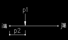
`p1`	Load P [N]
`p2`	Distance a from the i-end [mm]
`p3, p4`	Not used

A concentrated load at an arbitrary point along the member (unlike a nodal load, it acts within the member)

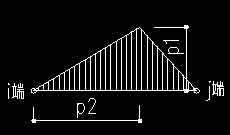
Type 2: Triangular distribution (zero at both ends, arbitrary peak)

`p1`	Peak w [N/mm]
`p2`	Peak position a [mm] (0 = midspan, same as Type 4)
`p3, p4`	Not used

Zero at both ends with a peak of w at position a. With p2 = 0 the peak is at midspan (same shape as Type 4)

Type 3: Trapezoidal distribution

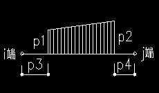
`p1`	w at the i-end [N/mm]
`p2`	w at the j-end [N/mm]
`p3`	Offset p3 from the i-end [mm]
`p4`	Offset p4 from the j-end [mm]

Set p1 = p2 for a uniform load. With p3 = p4 = 0 the load covers the full length

Type 4: Triangular (peak at midspan)

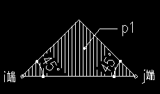
`p1`	Peak intensity w [N/mm]
`p2–p4`	Not used

Isosceles triangular distribution: maximum at midspan, zero at both ends. Same shape as Type 2 with p2 = 0 (midspan)

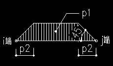
Type 5: Trapezoid with ramps at both ends

`p1`	Peak intensity w [N/mm]
`p2`	Ramp length at both ends [mm]
`p3, p4`	Not used

Constant w in the middle, dropping linearly to zero over length p2 at each end

Types 6 (ramp up) and 7 (ramp down) are not included in the current UI choices (the internal code is retained).

4.7 Prescribed Displacements

Applies prescribed displacements to restrained degrees of freedom — used for support settlement, imposed rotation, and the like.

Column	Description
`Node`	Node ID to which the displacement is applied
`δx`	Prescribed displacement in X [mm]
`δy`	Prescribed displacement in Y [mm] (settlement is negative)
`θz`	Prescribed rotation about Z [rad]

Important: For a prescribed displacement to take effect, the corresponding direction must be restrained (☑) in the Nodes table.
Example: support settlement δy = −2 mm → set dy = ☑ on the node and enter δy = −2.
Example: imposed rotation θz = 0.2 rad → set rz = ☑ on the node and enter θz = 0.2.
Values specified on free (unrestrained) nodes are ignored.

Analysis theory: The partition method is used. For prescribed displacements Uc, the tool solves Kff · Uf = Ff − Kfc · Uc, so the specified values are reflected exactly in displacements, reactions and internal forces.

5. View Panel

Structural model view

Element	Color / shape
Nodes	Blue circles (with the node ID)
Members	Black lines (member ID at midspan)
Pinned connection	Small white circle at the member end
Fixed support	Black hatched block
Pin support	Triangle (red)
Roller support	Triangle (green)
Nodal loads	Blue arrows
Member loads	Multiple blue arrows with a dashed envelope
Reactions (after analysis)	Red arrows
Coordinate axes	X and Y directions shown in the lower-left corner
Dimension lines	Horizontal and vertical model dimensions shown faintly at the edges

Deformed shape

Shows the deformed shape after analysis; the original shape is drawn faintly. Deformation is interpolated with Bezier curves (Euler–Bernoulli beam theory).

Item	Description
Top-left label	`Max nodal disp. = ○○ [mm]` (largest displacement magnitude among all nodes)
Max displacement marker	Orange ring and value at the node(s) with the maximum displacement
Midspan displacement	Bezier midpoint displacement of members inclined ≤ 45° shown as `δ=○○`
Bottom-left label	`Deformation scale ×n`. Zoom buttons double or halve the scale

Force diagrams

Switch between the M, Q and N diagrams. Positive and negative values are drawn in different colors.

Item	Description
End labels	Numeric force values at the i-end and j-end
Midspan M label	M diagram only: midspan moment value shown for members inclined ≤ 45°
Top-left label	`M diagram max=○○ [N·mm]` / `Q diagram max=○○ [N]` / `N diagram max=○○ [N]`

Note: The Deformed Shape and Force Diagram tabs are grayed out and unclickable until an analysis has been run. They become available after "Run Analysis".

6. Reading the Analysis Results

After running the analysis, results appear in the panel at the lower right. The "Font size: S M L" buttons at the right of the header change the text size (the setting is saved in your browser).

Nodal displacements

Column	Description
Node	Node ID
δx [mm]	Displacement in X
δy [mm]	Displacement in Y
θz [rad]	Rotation about the Z axis

Reactions

Column	Description
Node	Support node ID
Rx [N]	Reaction in X (positive to the right)
Ry [N]	Reaction in Y (positive upward)
Rm [N·mm]	Moment reaction (CCW positive)

Verification: Check that ΣFx = 0, ΣFy = 0 and ΣM = 0 hold.

Member end forces

Column	Description
Member	Member ID
End	i-end (start) or j-end (end)
N [N]	Axial force (tension positive)
Q [N]	Shear force
M [N·mm]	Bending moment (CCW positive)

7. Saving and Loading Data

Feature	Description
Auto-save	Saved to localStorage after every change; restored even after closing the page
Save Input Data	Downloads the model as `strlab_model.json` (toolbar, right side)
Load Input Data	Restores a previously saved JSON file and re-runs the analysis automatically (toolbar, right side)
Reset	Restores the default portal frame model (with a confirmation dialog)

Note: Clearing your browser's site data deletes the localStorage copy. Export important models as JSON.

8. Analysis Settings (Units and Axial Deformation)

The "⚙ Settings" button at the right end of the toolbar opens the analysis settings dialog. The current settings are always shown to the left of the button, e.g. "Units: N·mm / Axial deformation: considered" (clicking that text also opens the dialog).

Setting	Choices	Description
Force unit	N / kN	Force unit for input values and results
Length unit	mm / cm	Length unit for input values and results
Axial deformation	Considered / Ignored	Whether axial elongation of members is ignored (see below)

How the unit setting works

Important: The unit setting declares how input values are interpreted — existing input values are not converted. Changing units while a model contains data therefore replaces it, after a confirmation dialog, with the initial model in the new unit system. Decide on the unit system before you start entering data.

Input table headers (e.g. E [N/mm²]) and the units in the result tables switch automatically with the setting.
Loading a sample model resets the units to N·mm (samples are defined in the N·mm system). The axial deformation setting is preserved.
The unit setting is stored as part of the model data in localStorage and in exported JSON.

Ignoring axial deformation

Selecting "Axial deformation: ignored" performs the analysis with axial elongation of members suppressed — handy for comparing against hand-calculation methods that neglect column shortening (moment distribution, D-value method, etc.). Internally a penalty method treats the axial stiffness as effectively infinite. See the Theory of Computation for details.

Note: Changing the axial deformation setting does not automatically re-run the analysis. Always press "▶ Run Analysis" again after changing it.

9. Analysis Theory (Summary)

This tool performs linear elastic analysis using the direct stiffness method. The computation proceeds as follows.

Build the local stiffness matrix (6×6) for each member (pinned ends handled by static condensation)
Transform to global coordinates and assemble into the global stiffness matrix K
Build the load vector F from nodal loads and equivalent nodal forces converted from member loads
Handle support conditions and prescribed displacements with the partition method (K_ff·U_f = F_f − K_fc·U_c)
Solve for nodal displacements by Gaussian elimination with partial pivoting
Compute reactions, member end forces and internal force diagrams

▶ For details, see the Theory of Computation page.
It covers the stiffness matrix components, equivalent nodal force formulas, pin-end corrections, the partition method for prescribed displacements, the penalty method for ignoring axial deformation, and verification examples against theoretical solutions.

10. Sign Conventions

Global coordinate system: Y↑ │ └──────→ X Z (out of plane): positive toward the viewer (right-handed) θ: counterclockwise (CCW) positive Member local coordinates: Y_local ↑ │ i-end ────────┼────────── j-end X_local → X_local: direction from the i-end to the j-end Y_local: X_local rotated 90° counterclockwise Positive internal forces: N (axial force) : tension positive Q (shear force) : downward on the right face at the i-end positive M (bending moment): CCW positive

11. Notes and Limitations

Linear elastic analysis only — plasticity, geometric nonlinearity and buckling are not covered.
Use consistent units — mm, N and N/mm² are recommended. Mixing units produces wrong results.
Minimum restraints are required — the supports must restrain ΣFx, ΣFy and ΣM.
Truss analysis — set all members to pinned at both ends (□□) and use only nodal loads to analyze a pure truss.
Self-weight is not computed automatically — convert it manually into member or nodal loads.
Numerical precision — models mixing members with extremely different stiffness ratios (EA/EI) can become numerically unstable.
Sign of member loads (downward loads) — the coordinate system is positive-Y-up. Enter negative p1 (e.g. p1 = −5) for gravity-direction (downward) loads.
Activating prescribed displacements — to impose settlement or similar, restrain the target DOF (dx/dy/rz with ☑) and then enter the prescribed value. Values entered while the restraint flag is □ are not reflected in the analysis.

12. Input Examples

Example 1: Cantilever beam (10 kN concentrated load at the free end)

Node N1	x=0, y=0, dx=☑, dy=☑, rz=☑ (fixed end)
Node N2	x=3000, y=0, dx=□, dy=□, rz=□ (free end)
Material M1	E=205000 [N/mm²]
Section S1	A=6353, I=47200000 (≈ H-200×200)
Member B1	N1→N2, M1, S1, rigid at both ends
Nodal load	N2: Py = −10000 [N] (downward)

Fixed-end moment (theory): M = P × L = 10,000 × 3,000 = 30,000,000 N·mm

Example 2: Simply supported beam (uniform downward load w = 1.0 N/mm)

Node N1	x=0, y=0, dx=☑, dy=☑ (pin support)
Node N2	x=6000, y=0, dy=☑ (roller support)
Member B1	N1→N2, rigid at both ends
Member load	Member=B1, Type=3, Dir=1, p1=−1.0, p2=−1.0, p3=0, p4=0

Maximum midspan moment (theory): M = w × L² / 8 = 1.0 × 6,000² / 8 = 4,500,000 N·mm
* Because the Y axis is positive upward, enter negative p1 for downward loads.

Example 3: Portal frame (default model)

The default model shown when the page loads is a basic portal frame with fixed supports at both bases, two columns and one beam. A horizontal concentrated load of 10 N acts on the upper-left node.

Example 4: Support settlement (roller support settles 5 mm)

Node N1	x=0, y=0, dx=☑, dy=☑ (pin support)
Node N2	x=6000, y=0, dy=☑ (roller support)
Prescribed disp.	Node=N2, δy=−5 [mm] (downward settlement)

Set dy of N2 to ☑ (restrained), then enter δy = −5 in the Prescribed Displacements tab.
The prescribed displacement is not reflected in the analysis while the restraint flag is □.

Example 5: Sample models (portal frames)

The "Select a sample…" dropdown in the toolbar instantly loads portal frames from 1 story × 1 bay up to 3 stories × 3 bays. Every horizontal member carries a downward trapezoidal load (Type 5, p1 = −5 N/mm, p2 = 1500 mm).